3.2 Fluid Flow Relationships

The study of fluid dynamics is largely driven by mathematical relationships between different features of the fluid flow. This lesson builds on the concepts from Lesson 3.1 Fluid Transport PhenomenaA field of engineering that studies mass, energy, and momentum within and between systems Fundamentals, introducing some equations to describe fluid flow and classify said flows according to their flow regime.

Fluid Dynamics Between Parallel Plates

Lesson 3.1 Fluid Transport Phenomena Fundamentals introduced the concept of Newtonian and non-Newtonian fluids, which can be identified and classified by applying stresses and analysing the reacting. Figure 1 is a parallel plate diagram which can be used to demonstrate this.

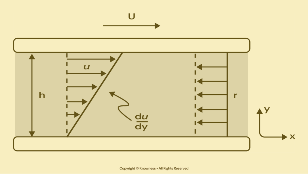
Taking the parallel plates shown, if the gap between the plates is filled by a Newtonian fluidA fluid that obeys Newton’s Law of Viscosity. and the top plate is moved at a constant velocity, the fluid will deform linearly. The molecules adjacent to a plate, either the top or bottom, move at the same velocity as the plate, which is called the non-slip boundary condition. The velocity at the top is ‘U’ and the velocity at the stationary bottom plate is zero, resulting in a linear velocity profile described by the velocity gradient du/dy. This velocity gradient is also known as the shear rate.

Measuring the force required to move the top plate at the velocity ‘U’ and multiplying by the area of the plate gives the shear stress. Isaac Newton found that the shear stress and shear rate can be linearly related using a constant called dynamic viscosity, thus giving Newton’s Law of Viscosity, shown in Equation 1.